Physics and Equation-Based Modeling Interfaces
Using COMSOL Multiphysics provides you with a significant amount of physics modeling functionality, including multiphysics ability. By adding application-specific modules, the modeling power is increased with dedicated tools for electrical, mechanical, fluid flow, and chemical applications. COMSOL Multiphysics includes a set of core physics interfaces for common physics application areas such as structural analysis, laminar flow, pressure acoustics, transport of diluted species, electrostatics, electric currents, heat transfer, and Joule heating. These are simplified versions of a selected set of physics interfaces available in the add-on modules.
For arbitrary mathematics or physics simulations, where a preset physics option is not available, a set of physics interfaces are included for setting up simulations from first principles by defining the equations. Several partial differential equation (PDE) templates make it easy to model second-order linear or nonlinear systems of equations. By stacking several equations together, you can also model higher-order differential equations. These equation-based tools can further be combined with the preset physics of COMSOL Multiphysics or any of the add-on modules, allowing for fully-coupled and customized analyses. This dramatically reduces the need for writing user subroutines in order to customize equations, material properties, boundary conditions, or source terms. Also available is a set of templates for classical PDEs: Laplace's equation, Poisson's equation, the wave equation, the Helmholtz equation, the heat equation, and the convection-diffusion equation.
Coordinate Systems
Users enjoy the ability to define any number of local coordinate systems. There are shortcuts for common coordinate systems such as cylindrical, spherical, and Euler-angle based, and a method for automatic coordinate system creation makes it easy to define anisotropic material properties that follow curved geometric shapes. This curvilinear coordinates tool, included in COMSOL Multiphysics, can be applied for any type of physics, like anisotropic thermal conductivity in heat transfer, orthotropic materials for structural mechanics, and anisotropic media in electromagnetics, for example.
Model Couplings
The COMSOL Desktop® allows you to work simultaneously in 3D, 2D, 1D, and 0D. So called Model Couplings can be used to map any quantity across spatial dimensions. For example, a 2D solution can be mapped to a 3D surface or extruded throughout a 3D volume. This functionality makes it easy to set up cross-dimensional simulations. Furthermore, systems of algebraic equations, ordinary differential equations (ODEs), or differential algebraic equations (DAEs) – referred to as 0D models – can be combined with spatially dependent 1D, 2D, and 3D models.
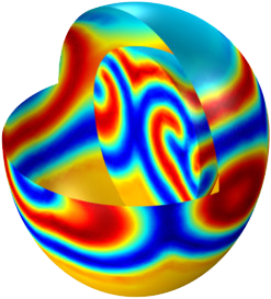 Partial Differential Equations: An equation-based model of electrical signals in a heart, solving a system of transient nonlinear partial differential equations.
Partial Differential Equations: An equation-based model of electrical signals in a heart, solving a system of transient nonlinear partial differential equations.
View Additional Screenshots »
Moving Mesh with ALE
COMSOL Multiphysics includes advanced moving mesh functionality, based on the Arbitrary Lagrangian-Eulerian (ALE) method, where you can define physics with respect to a moving frame of reference. This can be either a material frame or a spatial frame depending on what is relevant for the physics at hand. The technology is also included in some of the add-on modules, where moving meshes are coupled to other physics: fluid-structure interaction (Structural Mechanics Module and MEMS Module), corroding surfaces (Corrosion Module), electrodeposition (Electrodeposition Module), electromechanics (MEMS Module), and two-phase flow (Microfluidics Module). The ALE functionality included in COMSOL Multiphysics also makes it possible to perform custom-built simulations in cases where a built-in option is not available.

")